gageRR-class: Class `gageRR`

R6 Class for Gage R&R (Repeatability and Reproducibility) Analysis

Public fields

X: Data frame containing the measurement data.
ANOVA: List containing the results of the Analysis of Variance (ANOVA) for the gage study.
RedANOVA: List containing the results of the reduced ANOVA.
method: Character string specifying the method used for the analysis (e.g., `crossed`, `nested`).
Estimates: List of estimates including variance components, repeatability, and reproducibility.
Varcomp: List of variance components.
Sigma: Numeric value representing the standard deviation of the measurement system.
GageName: Character string representing the name of the gage.
GageTolerance: Numeric value indicating the tolerance of the gage.
DateOfStudy: Character string representing the date of the gage R&R study.
PersonResponsible: Character string indicating the person responsible for the study.
Comments: Character string for additional comments or notes about the study.
b: Factor levels for operator.
a: Factor levels for part.
y: Numeric vector or matrix containing the measurement responses.
facNames: Character vector specifying the names of the factors (e.g., `Operator`, `Part`).
numO: Integer representing the number of operators.
numP: Integer representing the number of parts.
numM: Integer representing the number of measurements per part-operator combination.

Methods

Public methods

gageRR.c$new()
gageRR.c$print()
gageRR.c$subset()
gageRR.c$summary()
gageRR.c$get.response()
gageRR.c$response()
gageRR.c$names()
gageRR.c$as.data.frame()
gageRR.c$get.tolerance()
gageRR.c$set.tolerance()
gageRR.c$get.sigma()
gageRR.c$set.sigma()
gageRR.c$plot()
gageRR.c$errorPlot()
gageRR.c$whiskersPlot()
gageRR.c$averagePlot()
gageRR.c$compPlot()
gageRR.c$clone()

Method `new()`

Initialize the fiels of the gageRR object

Usage

gageRR.c$new(
  X,
  ANOVA = NULL,
  RedANOVA = NULL,
  method = NULL,
  Estimates = NULL,
  Varcomp = NULL,
  Sigma = NULL,
  GageName = NULL,
  GageTolerance = NULL,
  DateOfStudy = NULL,
  PersonResponsible = NULL,
  Comments = NULL,
  b = NULL,
  a = NULL,
  y = NULL,
  facNames = NULL,
  numO = NULL,
  numP = NULL,
  numM = NULL
)

Arguments

X: Data frame containing the measurement data.
ANOVA: List containing the results of the Analysis of Variance (ANOVA) for the gage study.
RedANOVA: List containing the results of the reduced ANOVA.
method: Character string specifying the method used for the analysis (e.g., "crossed", "nested").
Estimates: List of estimates including variance components, repeatability, and reproducibility.
Varcomp: List of variance components.
Sigma: Numeric value representing the standard deviation of the measurement system.
GageName: Character string representing the name of the gage.
GageTolerance: Numeric value indicating the tolerance of the gage.
DateOfStudy: Character string representing the date of the gage R&R study.
PersonResponsible: Character string indicating the person responsible for the study.
Comments: Character string for additional comments or notes about the study.
b: Factor levels for operator.
a: Factor levels for part.
y: Numeric vector or matrix containing the measurement responses.
facNames: Character vector specifying the names of the factors (e.g., "Operator", "Part").
numO: Integer representing the number of operators.
numP: Integer representing the number of parts.
numM: Integer representing the number of measurements per part-operator combination.

Method `print()`

Return the data frame containing the measurement data (X)

Usage

gageRR.c$print()

Method `subset()`

Return a subset of the data frame that containing the measurement data (X)

Usage

gageRR.c$subset(i, j)

Arguments

i: The i-position of the row of X.
j: The j-position of the column of X.

Method `summary()`

Summarize the information of the fields of the gageRR object.

Usage

gageRR.c$summary()

Method `get.response()`

Get or get the response for a gageRRDesign object.

Usage

gageRR.c$get.response()

Method `response()`

Set the response for a gageRRDesign object.

Usage

gageRR.c$response(value)

Arguments

value: New response vector.

Method `names()`

Methods for function names in Package base.

Usage

gageRR.c$names()

Method `as.data.frame()`

Methods for function as.data.frame in Package base.

Usage

gageRR.c$as.data.frame()

Method `get.tolerance()`

Get the tolerance for an object of class gageRR.

Usage

gageRR.c$get.tolerance()

Method `set.tolerance()`

Set the tolerance for an object of class gageRR.

Usage

gageRR.c$set.tolerance(value)

Arguments

value: A data.frame or vector for the new value of tolerance.

Method `get.sigma()`

Get the sigma for an object of class gageRR.

Usage

gageRR.c$get.sigma()

Method `set.sigma()`

Set the sigma for an object of class gageRR.

Usage

gageRR.c$set.sigma(value)

Arguments

value: Valor of sigma

Method `plot()`

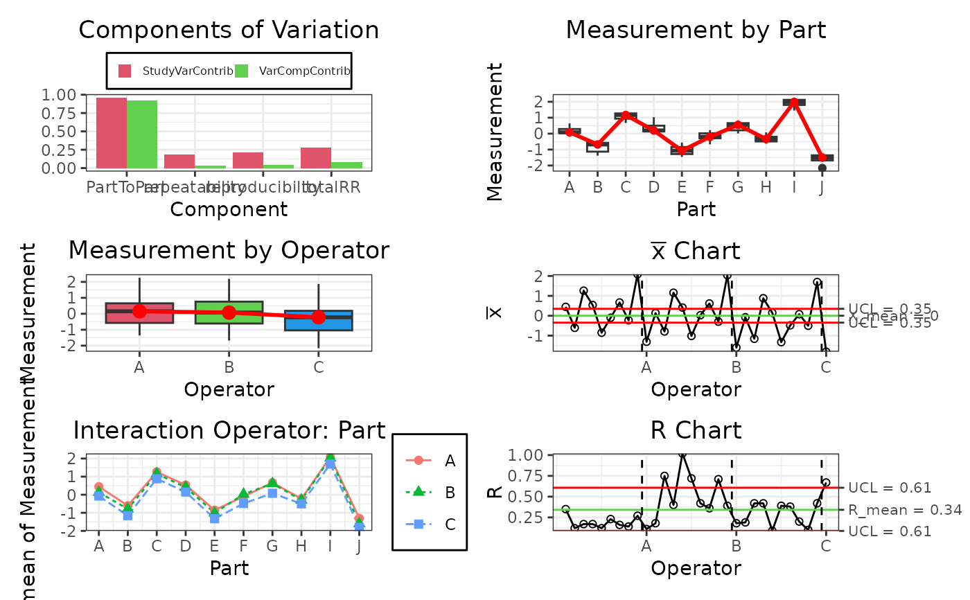
This function creates a customized plot using the data from the gageRR.c object.

Usage

gageRR.c$plot(main = NULL, xlab = NULL, ylab = NULL, col, lwd, fun = mean)

Arguments

main: Character string specifying the title of the plot.
xlab: A character string for the x-axis label.
ylab: A character string for the y-axis label.
col: A character string or vector specifying the color(s) to be used for the plot elements.
lwd: A numeric value specifying the line width of plot elements
fun: Function to use for the calculation of the interactions (e.g., mean, median). Default is mean.

Examples

# Create gageRR-object
gdo = gageRRDesign(Operators = 3, Parts = 10, Measurements = 3, randomize = FALSE)
# Vector of responses
y = c(0.29,0.08, 0.04,-0.56,-0.47,-1.38,1.34,1.19,0.88,0.47,0.01,0.14,-0.80,
      -0.56,-1.46, 0.02,-0.20,-0.29,0.59,0.47,0.02,-0.31,-0.63,-0.46,2.26,
      1.80,1.77,-1.36,-1.68,-1.49,0.41,0.25,-0.11,-0.68,-1.22,-1.13,1.17,0.94,
      1.09,0.50,1.03,0.20,-0.92,-1.20,-1.07,-0.11, 0.22,-0.67,0.75,0.55,0.01,
      -0.20, 0.08,-0.56,1.99,2.12,1.45,-1.25,-1.62,-1.77,0.64,0.07,-0.15,-0.58,
      -0.68,-0.96,1.27,1.34,0.67,0.64,0.20,0.11,-0.84,-1.28,-1.45,-0.21,0.06,
      -0.49,0.66,0.83,0.21,-0.17,-0.34,-0.49,2.01,2.19,1.87,-1.31,-1.50,-2.16)

# Appropriate responses
gdo$response(y)
# Perform and gageRR
gdo <- gageRR(gdo)

gdo$plot()

Method `errorPlot()`

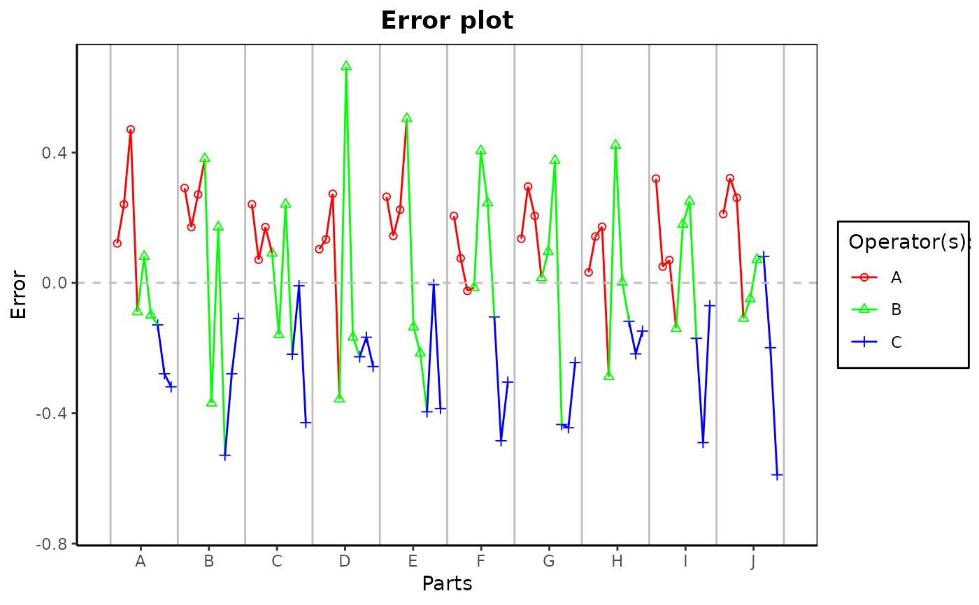
The data from an object of class gageRR can be analyzed by running `Error Charts` of the individual deviations from the accepted rference values. These `Error Charts` are provided by the function errorPlot.

Usage

gageRR.c$errorPlot(main, xlab, ylab, col, pch, ylim, legend = TRUE)

Arguments

main: a main title for the plot.
xlab: A character string for the x-axis label.
ylab: A character string for the y-axis label.
col: Plotting color.
pch: An integer specifying a symbol or a single character to be used as the default in plotting points.
ylim: The y limits of the plot.
legend: A logical value specifying whether a legend is plotted automatically. By default legend is set to `TRUE`.

Examples

# Create gageRR-object
gdo = gageRRDesign(Operators = 3, Parts = 10, Measurements = 3, randomize = FALSE)
# Vector of responses
y = c(0.29,0.08, 0.04,-0.56,-0.47,-1.38,1.34,1.19,0.88,0.47,0.01,0.14,-0.80,
      -0.56,-1.46, 0.02,-0.20,-0.29,0.59,0.47,0.02,-0.31,-0.63,-0.46,2.26,
      1.80,1.77,-1.36,-1.68,-1.49,0.41,0.25,-0.11,-0.68,-1.22,-1.13,1.17,0.94,
      1.09,0.50,1.03,0.20,-0.92,-1.20,-1.07,-0.11, 0.22,-0.67,0.75,0.55,0.01,
      -0.20, 0.08,-0.56,1.99,2.12,1.45,-1.25,-1.62,-1.77,0.64,0.07,-0.15,-0.58,
      -0.68,-0.96,1.27,1.34,0.67,0.64,0.20,0.11,-0.84,-1.28,-1.45,-0.21,0.06,
      -0.49,0.66,0.83,0.21,-0.17,-0.34,-0.49,2.01,2.19,1.87,-1.31,-1.50,-2.16)

# Appropriate responses
gdo$response(y)
# Perform and gageRR
gdo <- gageRR(gdo)

gdo$errorPlot()

Method `whiskersPlot()`

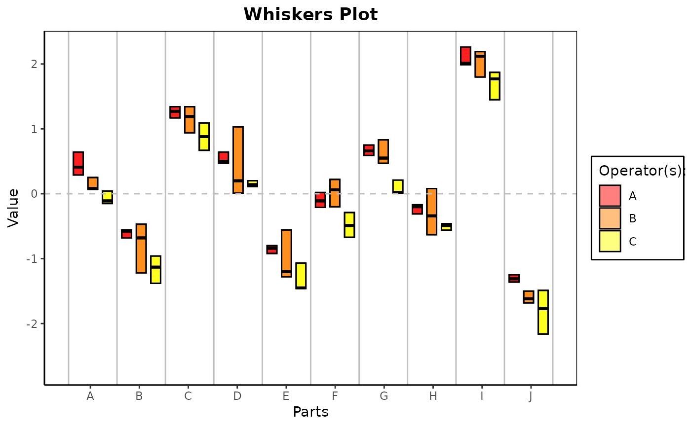
In a Whiskers Chart, the high and low data values and the average (median) by part-by-operator are plotted to provide insight into the consistency between operators, to indicate outliers and to discover part-operator interactions. The Whiskers Chart reminds of boxplots for every part and every operator.

Usage

gageRR.c$whiskersPlot(main, xlab, ylab, col, ylim, legend = TRUE)

Arguments

main: a main title for the plot.
xlab: A character string for the x-axis label.
ylab: A character string for the y-axis label.
col: Plotting color.
ylim: The y limits of the plot.
legend: A logical value specifying whether a legend is plotted automatically. By default legend is set to `TRUE`.

Examples

# Create gageRR-object
gdo = gageRRDesign(Operators = 3, Parts = 10, Measurements = 3, randomize = FALSE)
# Vector of responses
y = c(0.29,0.08, 0.04,-0.56,-0.47,-1.38,1.34,1.19,0.88,0.47,0.01,0.14,-0.80,
      -0.56,-1.46, 0.02,-0.20,-0.29,0.59,0.47,0.02,-0.31,-0.63,-0.46,2.26,
      1.80,1.77,-1.36,-1.68,-1.49,0.41,0.25,-0.11,-0.68,-1.22,-1.13,1.17,0.94,
      1.09,0.50,1.03,0.20,-0.92,-1.20,-1.07,-0.11, 0.22,-0.67,0.75,0.55,0.01,
      -0.20, 0.08,-0.56,1.99,2.12,1.45,-1.25,-1.62,-1.77,0.64,0.07,-0.15,-0.58,
      -0.68,-0.96,1.27,1.34,0.67,0.64,0.20,0.11,-0.84,-1.28,-1.45,-0.21,0.06,
      -0.49,0.66,0.83,0.21,-0.17,-0.34,-0.49,2.01,2.19,1.87,-1.31,-1.50,-2.16)

# Appropriate responses
gdo$response(y)
# Perform and gageRR
gdo <- gageRR(gdo)

gdo$whiskersPlot()

Method `averagePlot()`

averagePlot creates all x-y plots of averages by size out of an object of class gageRR. Therfore the averages of the multiple readings by each operator on each part are plotted with the reference value or overall part averages as the index.

Usage

gageRR.c$averagePlot(main, xlab, ylab, col, single = FALSE)

Arguments

main: a main title for the plot.
xlab: A character string for the x-axis label.
ylab: A character string for the y-axis label.
col: Plotting color.
single: A logical value.If `TRUE` a new graphic device will be opened for each plot. By default single is set to `FALSE`.

Examples

# Create gageRR-object
gdo = gageRRDesign(Operators = 3, Parts = 10, Measurements = 3, randomize = FALSE)
# Vector of responses
y = c(0.29,0.08, 0.04,-0.56,-0.47,-1.38,1.34,1.19,0.88,0.47,0.01,0.14,-0.80,
      -0.56,-1.46, 0.02,-0.20,-0.29,0.59,0.47,0.02,-0.31,-0.63,-0.46,2.26,
      1.80,1.77,-1.36,-1.68,-1.49,0.41,0.25,-0.11,-0.68,-1.22,-1.13,1.17,0.94,
      1.09,0.50,1.03,0.20,-0.92,-1.20,-1.07,-0.11, 0.22,-0.67,0.75,0.55,0.01,
      -0.20, 0.08,-0.56,1.99,2.12,1.45,-1.25,-1.62,-1.77,0.64,0.07,-0.15,-0.58,
      -0.68,-0.96,1.27,1.34,0.67,0.64,0.20,0.11,-0.84,-1.28,-1.45,-0.21,0.06,
      -0.49,0.66,0.83,0.21,-0.17,-0.34,-0.49,2.01,2.19,1.87,-1.31,-1.50,-2.16)

# Appropriate responses
gdo$response(y)
# Perform and gageRR
gdo <- gageRR(gdo)

gdo$averagePlot()

Method `compPlot()`

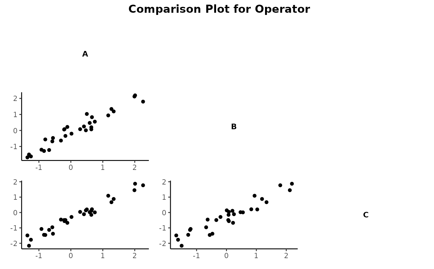
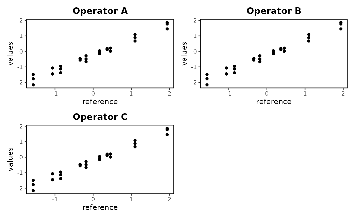
compPlot creates comparison x-y plots of an object of class gageRR. The averages of the multiple readings by each operator on each part are plotted against each other with the operators as indices. This plot compares the values obtained by one operator to those of another.

Usage

gageRR.c$compPlot(main, xlab, ylab, col, cex.lab, fun = NULL)

Arguments

main: a main title for the plot.
xlab: A character string for the x-axis label.
ylab: A character string for the y-axis label.
col: Plotting color.
cex.lab: The magnification to be used for x and y labels relative to the current setting of cex.
fun: Optional function that will be applied to the multiple readings of each part. fun should be an object of class function like mean,median, sum, etc. By default, fun is set to `NULL` and all readings will be plotted.

Examples

# Create gageRR-object
gdo = gageRRDesign(Operators = 3, Parts = 10, Measurements = 3, randomize = FALSE)
# Vector of responses
y = c(0.29,0.08, 0.04,-0.56,-0.47,-1.38,1.34,1.19,0.88,0.47,0.01,0.14,-0.80,
      -0.56,-1.46, 0.02,-0.20,-0.29,0.59,0.47,0.02,-0.31,-0.63,-0.46,2.26,
      1.80,1.77,-1.36,-1.68,-1.49,0.41,0.25,-0.11,-0.68,-1.22,-1.13,1.17,0.94,
      1.09,0.50,1.03,0.20,-0.92,-1.20,-1.07,-0.11, 0.22,-0.67,0.75,0.55,0.01,
      -0.20, 0.08,-0.56,1.99,2.12,1.45,-1.25,-1.62,-1.77,0.64,0.07,-0.15,-0.58,
      -0.68,-0.96,1.27,1.34,0.67,0.64,0.20,0.11,-0.84,-1.28,-1.45,-0.21,0.06,
      -0.49,0.66,0.83,0.21,-0.17,-0.34,-0.49,2.01,2.19,1.87,-1.31,-1.50,-2.16)

# Appropriate responses
gdo$response(y)
# Perform and gageRR
gdo <- gageRR(gdo)

gdo$compPlot()

Method `clone()`

The objects of this class are cloneable with this method.

Usage

gageRR.c$clone(deep = FALSE)

Arguments

deep: Whether to make a deep clone.

Examples

#create gageRR-object
gdo <- gageRRDesign(Operators = 3, Parts = 10, Measurements = 3, randomize = FALSE)
#vector of responses
y <- c(0.29,0.08, 0.04,-0.56,-0.47,-1.38,1.34,1.19,0.88,0.47,0.01,0.14,-0.80,
      -0.56,-1.46, 0.02,-0.20,-0.29,0.59,0.47,0.02,-0.31,-0.63,-0.46,2.26,
      1.80,1.77,-1.36,-1.68,-1.49,0.41,0.25,-0.11,-0.68,-1.22,-1.13,1.17,0.94,
      1.09,0.50,1.03,0.20,-0.92,-1.20,-1.07,-0.11, 0.22,-0.67,0.75,0.55,0.01,
      -0.20, 0.08,-0.56,1.99,2.12,1.45,-1.25,-1.62,-1.77,0.64,0.07,-0.15,-0.58,
      -0.68,-0.96,1.27,1.34,0.67,0.64,0.20,0.11,-0.84,-1.28,-1.45,-0.21,0.06,
      -0.49,0.66,0.83,0.21,-0.17,-0.34,-0.49,2.01,2.19,1.87,-1.31,-1.50,-2.16)

#appropriate responses
gdo$response(y)
# perform and gageRR
gdo <- gageRR(gdo)
#> 
#> AnOVa Table -  crossed Design
#>               Df Sum Sq Mean Sq F value   Pr(>F)    
#> Operator       2   3.17   1.584  34.440 1.09e-10 ***
#> Part           9  88.36   9.818 213.517  < 2e-16 ***
#> Operator:Part 18   0.36   0.020   0.434    0.974    
#> Residuals     60   2.76   0.046                     
#> ---
#> Signif. codes:  0 ‘***’ 0.001 ‘**’ 0.01 ‘*’ 0.05 ‘.’ 0.1 ‘ ’ 1
#> 
#> ----------
#> AnOVa Table Without Interaction -  crossed Design
#>             Df Sum Sq Mean Sq F value   Pr(>F)    
#> Operator     2   3.17   1.584   39.62 1.34e-12 ***
#> Part         9  88.36   9.818  245.61  < 2e-16 ***
#> Residuals   78   3.12   0.040                     
#> ---
#> Signif. codes:  0 ‘***’ 0.001 ‘**’ 0.01 ‘*’ 0.05 ‘.’ 0.1 ‘ ’ 1
#> 
#> ----------
#> 
#> Gage R&R
#>                  VarComp VarCompContrib Stdev StudyVar StudyVarContrib
#> totalRR           0.0914         0.0776 0.302     1.81           0.279
#>  repeatability    0.0400         0.0339 0.200     1.20           0.184
#>  reproducibility  0.0515         0.0437 0.227     1.36           0.209
#>    Operator       0.0515         0.0437 0.227     1.36           0.209
#>    Operator:Part  0.0000         0.0000 0.000     0.00           0.000
#> Part to Part      1.0864         0.9224 1.042     6.25           0.960
#> totalVar          1.1779         1.0000 1.085     6.51           1.000
#> 
#> ---
#>  * Contrib equals Contribution in %
#>  **Number of Distinct Categories (truncated signal-to-noise-ratio) = 4 
#> 

# Using the plots
gdo$plot()


## ------------------------------------------------
## Method `gageRR.c$plot`
## ------------------------------------------------

# Create gageRR-object
gdo = gageRRDesign(Operators = 3, Parts = 10, Measurements = 3, randomize = FALSE)
# Vector of responses
y = c(0.29,0.08, 0.04,-0.56,-0.47,-1.38,1.34,1.19,0.88,0.47,0.01,0.14,-0.80,
      -0.56,-1.46, 0.02,-0.20,-0.29,0.59,0.47,0.02,-0.31,-0.63,-0.46,2.26,
      1.80,1.77,-1.36,-1.68,-1.49,0.41,0.25,-0.11,-0.68,-1.22,-1.13,1.17,0.94,
      1.09,0.50,1.03,0.20,-0.92,-1.20,-1.07,-0.11, 0.22,-0.67,0.75,0.55,0.01,
      -0.20, 0.08,-0.56,1.99,2.12,1.45,-1.25,-1.62,-1.77,0.64,0.07,-0.15,-0.58,
      -0.68,-0.96,1.27,1.34,0.67,0.64,0.20,0.11,-0.84,-1.28,-1.45,-0.21,0.06,
      -0.49,0.66,0.83,0.21,-0.17,-0.34,-0.49,2.01,2.19,1.87,-1.31,-1.50,-2.16)

# Appropriate responses
gdo$response(y)
# Perform and gageRR
gdo <- gageRR(gdo)
#> 
#> AnOVa Table -  crossed Design
#>               Df Sum Sq Mean Sq F value   Pr(>F)    
#> Operator       2   3.17   1.584  34.440 1.09e-10 ***
#> Part           9  88.36   9.818 213.517  < 2e-16 ***
#> Operator:Part 18   0.36   0.020   0.434    0.974    
#> Residuals     60   2.76   0.046                     
#> ---
#> Signif. codes:  0 ‘***’ 0.001 ‘**’ 0.01 ‘*’ 0.05 ‘.’ 0.1 ‘ ’ 1
#> 
#> ----------
#> AnOVa Table Without Interaction -  crossed Design
#>             Df Sum Sq Mean Sq F value   Pr(>F)    
#> Operator     2   3.17   1.584   39.62 1.34e-12 ***
#> Part         9  88.36   9.818  245.61  < 2e-16 ***
#> Residuals   78   3.12   0.040                     
#> ---
#> Signif. codes:  0 ‘***’ 0.001 ‘**’ 0.01 ‘*’ 0.05 ‘.’ 0.1 ‘ ’ 1
#> 
#> ----------
#> 
#> Gage R&R
#>                  VarComp VarCompContrib Stdev StudyVar StudyVarContrib
#> totalRR           0.0914         0.0776 0.302     1.81           0.279
#>  repeatability    0.0400         0.0339 0.200     1.20           0.184
#>  reproducibility  0.0515         0.0437 0.227     1.36           0.209
#>    Operator       0.0515         0.0437 0.227     1.36           0.209
#>    Operator:Part  0.0000         0.0000 0.000     0.00           0.000
#> Part to Part      1.0864         0.9224 1.042     6.25           0.960
#> totalVar          1.1779         1.0000 1.085     6.51           1.000
#> 
#> ---
#>  * Contrib equals Contribution in %
#>  **Number of Distinct Categories (truncated signal-to-noise-ratio) = 4 
#> 

gdo$plot()


## ------------------------------------------------
## Method `gageRR.c$errorPlot`
## ------------------------------------------------

# Create gageRR-object
gdo = gageRRDesign(Operators = 3, Parts = 10, Measurements = 3, randomize = FALSE)
# Vector of responses
y = c(0.29,0.08, 0.04,-0.56,-0.47,-1.38,1.34,1.19,0.88,0.47,0.01,0.14,-0.80,
      -0.56,-1.46, 0.02,-0.20,-0.29,0.59,0.47,0.02,-0.31,-0.63,-0.46,2.26,
      1.80,1.77,-1.36,-1.68,-1.49,0.41,0.25,-0.11,-0.68,-1.22,-1.13,1.17,0.94,
      1.09,0.50,1.03,0.20,-0.92,-1.20,-1.07,-0.11, 0.22,-0.67,0.75,0.55,0.01,
      -0.20, 0.08,-0.56,1.99,2.12,1.45,-1.25,-1.62,-1.77,0.64,0.07,-0.15,-0.58,
      -0.68,-0.96,1.27,1.34,0.67,0.64,0.20,0.11,-0.84,-1.28,-1.45,-0.21,0.06,
      -0.49,0.66,0.83,0.21,-0.17,-0.34,-0.49,2.01,2.19,1.87,-1.31,-1.50,-2.16)

# Appropriate responses
gdo$response(y)
# Perform and gageRR
gdo <- gageRR(gdo)
#> 
#> AnOVa Table -  crossed Design
#>               Df Sum Sq Mean Sq F value   Pr(>F)    
#> Operator       2   3.17   1.584  34.440 1.09e-10 ***
#> Part           9  88.36   9.818 213.517  < 2e-16 ***
#> Operator:Part 18   0.36   0.020   0.434    0.974    
#> Residuals     60   2.76   0.046                     
#> ---
#> Signif. codes:  0 ‘***’ 0.001 ‘**’ 0.01 ‘*’ 0.05 ‘.’ 0.1 ‘ ’ 1
#> 
#> ----------
#> AnOVa Table Without Interaction -  crossed Design
#>             Df Sum Sq Mean Sq F value   Pr(>F)    
#> Operator     2   3.17   1.584   39.62 1.34e-12 ***
#> Part         9  88.36   9.818  245.61  < 2e-16 ***
#> Residuals   78   3.12   0.040                     
#> ---
#> Signif. codes:  0 ‘***’ 0.001 ‘**’ 0.01 ‘*’ 0.05 ‘.’ 0.1 ‘ ’ 1
#> 
#> ----------
#> 
#> Gage R&R
#>                  VarComp VarCompContrib Stdev StudyVar StudyVarContrib
#> totalRR           0.0914         0.0776 0.302     1.81           0.279
#>  repeatability    0.0400         0.0339 0.200     1.20           0.184
#>  reproducibility  0.0515         0.0437 0.227     1.36           0.209
#>    Operator       0.0515         0.0437 0.227     1.36           0.209
#>    Operator:Part  0.0000         0.0000 0.000     0.00           0.000
#> Part to Part      1.0864         0.9224 1.042     6.25           0.960
#> totalVar          1.1779         1.0000 1.085     6.51           1.000
#> 
#> ---
#>  * Contrib equals Contribution in %
#>  **Number of Distinct Categories (truncated signal-to-noise-ratio) = 4 
#> 

gdo$errorPlot()


## ------------------------------------------------
## Method `gageRR.c$whiskersPlot`
## ------------------------------------------------

# Create gageRR-object
gdo = gageRRDesign(Operators = 3, Parts = 10, Measurements = 3, randomize = FALSE)
# Vector of responses
y = c(0.29,0.08, 0.04,-0.56,-0.47,-1.38,1.34,1.19,0.88,0.47,0.01,0.14,-0.80,
      -0.56,-1.46, 0.02,-0.20,-0.29,0.59,0.47,0.02,-0.31,-0.63,-0.46,2.26,
      1.80,1.77,-1.36,-1.68,-1.49,0.41,0.25,-0.11,-0.68,-1.22,-1.13,1.17,0.94,
      1.09,0.50,1.03,0.20,-0.92,-1.20,-1.07,-0.11, 0.22,-0.67,0.75,0.55,0.01,
      -0.20, 0.08,-0.56,1.99,2.12,1.45,-1.25,-1.62,-1.77,0.64,0.07,-0.15,-0.58,
      -0.68,-0.96,1.27,1.34,0.67,0.64,0.20,0.11,-0.84,-1.28,-1.45,-0.21,0.06,
      -0.49,0.66,0.83,0.21,-0.17,-0.34,-0.49,2.01,2.19,1.87,-1.31,-1.50,-2.16)

# Appropriate responses
gdo$response(y)
# Perform and gageRR
gdo <- gageRR(gdo)
#> 
#> AnOVa Table -  crossed Design
#>               Df Sum Sq Mean Sq F value   Pr(>F)    
#> Operator       2   3.17   1.584  34.440 1.09e-10 ***
#> Part           9  88.36   9.818 213.517  < 2e-16 ***
#> Operator:Part 18   0.36   0.020   0.434    0.974    
#> Residuals     60   2.76   0.046                     
#> ---
#> Signif. codes:  0 ‘***’ 0.001 ‘**’ 0.01 ‘*’ 0.05 ‘.’ 0.1 ‘ ’ 1
#> 
#> ----------
#> AnOVa Table Without Interaction -  crossed Design
#>             Df Sum Sq Mean Sq F value   Pr(>F)    
#> Operator     2   3.17   1.584   39.62 1.34e-12 ***
#> Part         9  88.36   9.818  245.61  < 2e-16 ***
#> Residuals   78   3.12   0.040                     
#> ---
#> Signif. codes:  0 ‘***’ 0.001 ‘**’ 0.01 ‘*’ 0.05 ‘.’ 0.1 ‘ ’ 1
#> 
#> ----------
#> 
#> Gage R&R
#>                  VarComp VarCompContrib Stdev StudyVar StudyVarContrib
#> totalRR           0.0914         0.0776 0.302     1.81           0.279
#>  repeatability    0.0400         0.0339 0.200     1.20           0.184
#>  reproducibility  0.0515         0.0437 0.227     1.36           0.209
#>    Operator       0.0515         0.0437 0.227     1.36           0.209
#>    Operator:Part  0.0000         0.0000 0.000     0.00           0.000
#> Part to Part      1.0864         0.9224 1.042     6.25           0.960
#> totalVar          1.1779         1.0000 1.085     6.51           1.000
#> 
#> ---
#>  * Contrib equals Contribution in %
#>  **Number of Distinct Categories (truncated signal-to-noise-ratio) = 4 
#> 

gdo$whiskersPlot()


## ------------------------------------------------
## Method `gageRR.c$averagePlot`
## ------------------------------------------------

# Create gageRR-object
gdo = gageRRDesign(Operators = 3, Parts = 10, Measurements = 3, randomize = FALSE)
# Vector of responses
y = c(0.29,0.08, 0.04,-0.56,-0.47,-1.38,1.34,1.19,0.88,0.47,0.01,0.14,-0.80,
      -0.56,-1.46, 0.02,-0.20,-0.29,0.59,0.47,0.02,-0.31,-0.63,-0.46,2.26,
      1.80,1.77,-1.36,-1.68,-1.49,0.41,0.25,-0.11,-0.68,-1.22,-1.13,1.17,0.94,
      1.09,0.50,1.03,0.20,-0.92,-1.20,-1.07,-0.11, 0.22,-0.67,0.75,0.55,0.01,
      -0.20, 0.08,-0.56,1.99,2.12,1.45,-1.25,-1.62,-1.77,0.64,0.07,-0.15,-0.58,
      -0.68,-0.96,1.27,1.34,0.67,0.64,0.20,0.11,-0.84,-1.28,-1.45,-0.21,0.06,
      -0.49,0.66,0.83,0.21,-0.17,-0.34,-0.49,2.01,2.19,1.87,-1.31,-1.50,-2.16)

# Appropriate responses
gdo$response(y)
# Perform and gageRR
gdo <- gageRR(gdo)
#> 
#> AnOVa Table -  crossed Design
#>               Df Sum Sq Mean Sq F value   Pr(>F)    
#> Operator       2   3.17   1.584  34.440 1.09e-10 ***
#> Part           9  88.36   9.818 213.517  < 2e-16 ***
#> Operator:Part 18   0.36   0.020   0.434    0.974    
#> Residuals     60   2.76   0.046                     
#> ---
#> Signif. codes:  0 ‘***’ 0.001 ‘**’ 0.01 ‘*’ 0.05 ‘.’ 0.1 ‘ ’ 1
#> 
#> ----------
#> AnOVa Table Without Interaction -  crossed Design
#>             Df Sum Sq Mean Sq F value   Pr(>F)    
#> Operator     2   3.17   1.584   39.62 1.34e-12 ***
#> Part         9  88.36   9.818  245.61  < 2e-16 ***
#> Residuals   78   3.12   0.040                     
#> ---
#> Signif. codes:  0 ‘***’ 0.001 ‘**’ 0.01 ‘*’ 0.05 ‘.’ 0.1 ‘ ’ 1
#> 
#> ----------
#> 
#> Gage R&R
#>                  VarComp VarCompContrib Stdev StudyVar StudyVarContrib
#> totalRR           0.0914         0.0776 0.302     1.81           0.279
#>  repeatability    0.0400         0.0339 0.200     1.20           0.184
#>  reproducibility  0.0515         0.0437 0.227     1.36           0.209
#>    Operator       0.0515         0.0437 0.227     1.36           0.209
#>    Operator:Part  0.0000         0.0000 0.000     0.00           0.000
#> Part to Part      1.0864         0.9224 1.042     6.25           0.960
#> totalVar          1.1779         1.0000 1.085     6.51           1.000
#> 
#> ---
#>  * Contrib equals Contribution in %
#>  **Number of Distinct Categories (truncated signal-to-noise-ratio) = 4 
#> 

gdo$averagePlot()


## ------------------------------------------------
## Method `gageRR.c$compPlot`
## ------------------------------------------------

# Create gageRR-object
gdo = gageRRDesign(Operators = 3, Parts = 10, Measurements = 3, randomize = FALSE)
# Vector of responses
y = c(0.29,0.08, 0.04,-0.56,-0.47,-1.38,1.34,1.19,0.88,0.47,0.01,0.14,-0.80,
      -0.56,-1.46, 0.02,-0.20,-0.29,0.59,0.47,0.02,-0.31,-0.63,-0.46,2.26,
      1.80,1.77,-1.36,-1.68,-1.49,0.41,0.25,-0.11,-0.68,-1.22,-1.13,1.17,0.94,
      1.09,0.50,1.03,0.20,-0.92,-1.20,-1.07,-0.11, 0.22,-0.67,0.75,0.55,0.01,
      -0.20, 0.08,-0.56,1.99,2.12,1.45,-1.25,-1.62,-1.77,0.64,0.07,-0.15,-0.58,
      -0.68,-0.96,1.27,1.34,0.67,0.64,0.20,0.11,-0.84,-1.28,-1.45,-0.21,0.06,
      -0.49,0.66,0.83,0.21,-0.17,-0.34,-0.49,2.01,2.19,1.87,-1.31,-1.50,-2.16)

# Appropriate responses
gdo$response(y)
# Perform and gageRR
gdo <- gageRR(gdo)
#> 
#> AnOVa Table -  crossed Design
#>               Df Sum Sq Mean Sq F value   Pr(>F)    
#> Operator       2   3.17   1.584  34.440 1.09e-10 ***
#> Part           9  88.36   9.818 213.517  < 2e-16 ***
#> Operator:Part 18   0.36   0.020   0.434    0.974    
#> Residuals     60   2.76   0.046                     
#> ---
#> Signif. codes:  0 ‘***’ 0.001 ‘**’ 0.01 ‘*’ 0.05 ‘.’ 0.1 ‘ ’ 1
#> 
#> ----------
#> AnOVa Table Without Interaction -  crossed Design
#>             Df Sum Sq Mean Sq F value   Pr(>F)    
#> Operator     2   3.17   1.584   39.62 1.34e-12 ***
#> Part         9  88.36   9.818  245.61  < 2e-16 ***
#> Residuals   78   3.12   0.040                     
#> ---
#> Signif. codes:  0 ‘***’ 0.001 ‘**’ 0.01 ‘*’ 0.05 ‘.’ 0.1 ‘ ’ 1
#> 
#> ----------
#> 
#> Gage R&R
#>                  VarComp VarCompContrib Stdev StudyVar StudyVarContrib
#> totalRR           0.0914         0.0776 0.302     1.81           0.279
#>  repeatability    0.0400         0.0339 0.200     1.20           0.184
#>  reproducibility  0.0515         0.0437 0.227     1.36           0.209
#>    Operator       0.0515         0.0437 0.227     1.36           0.209
#>    Operator:Part  0.0000         0.0000 0.000     0.00           0.000
#> Part to Part      1.0864         0.9224 1.042     6.25           0.960
#> totalVar          1.1779         1.0000 1.085     6.51           1.000
#> 
#> ---
#>  * Contrib equals Contribution in %
#>  **Number of Distinct Categories (truncated signal-to-noise-ratio) = 4 
#> 

gdo$compPlot()

Public fields

Methods

Public methods

Method new()

Usage

Arguments

Method print()

Usage

Method subset()

Usage

Arguments

Method summary()

Usage

Method get.response()

Usage

Method response()

Usage

Arguments

Method names()

Usage

Method as.data.frame()

Usage

Method get.tolerance()

Usage

Method set.tolerance()

Usage

Arguments

Method get.sigma()

Usage

Method set.sigma()

Usage

Arguments

Method plot()

Usage

Arguments

Examples

Method errorPlot()

Usage

Arguments

Examples

Method whiskersPlot()

Usage

Arguments

Examples

Method averagePlot()

Usage

Arguments

Examples

Method compPlot()

Usage

Arguments

Examples

Method clone()

Usage

Arguments

Examples

Method `new()`

Method `print()`

Method `subset()`

Method `summary()`

Method `get.response()`

Method `response()`

Method `names()`

Method `as.data.frame()`

Method `get.tolerance()`

Method `set.tolerance()`

Method `get.sigma()`

Method `set.sigma()`

Method `plot()`

Method `errorPlot()`

Method `whiskersPlot()`

Method `averagePlot()`

Method `compPlot()`

Method `clone()`